Nominal Regression in STAN
I was talking to a colleague about modeling nominal outcomes in STAN, and wrote up this example. Just put it here in case it’s helpful for anyone (probably myself in the future). This is based on an example I made for a course, where you can find the brms code for nominal regression. Please also check out the Multi-logit regression session on the Stan User’s guide.
Load Packages
library(cmdstanr)
library(dplyr)
library(ggplot2)
Check out this paper: https://journals.sagepub.com/doi/full/10.1177/2515245918823199
stemcell <- read.csv("https://osf.io/vxw73/download")stemcell |>
ggplot(aes(x = rating)) +
geom_bar() +
facet_wrap(~ gender)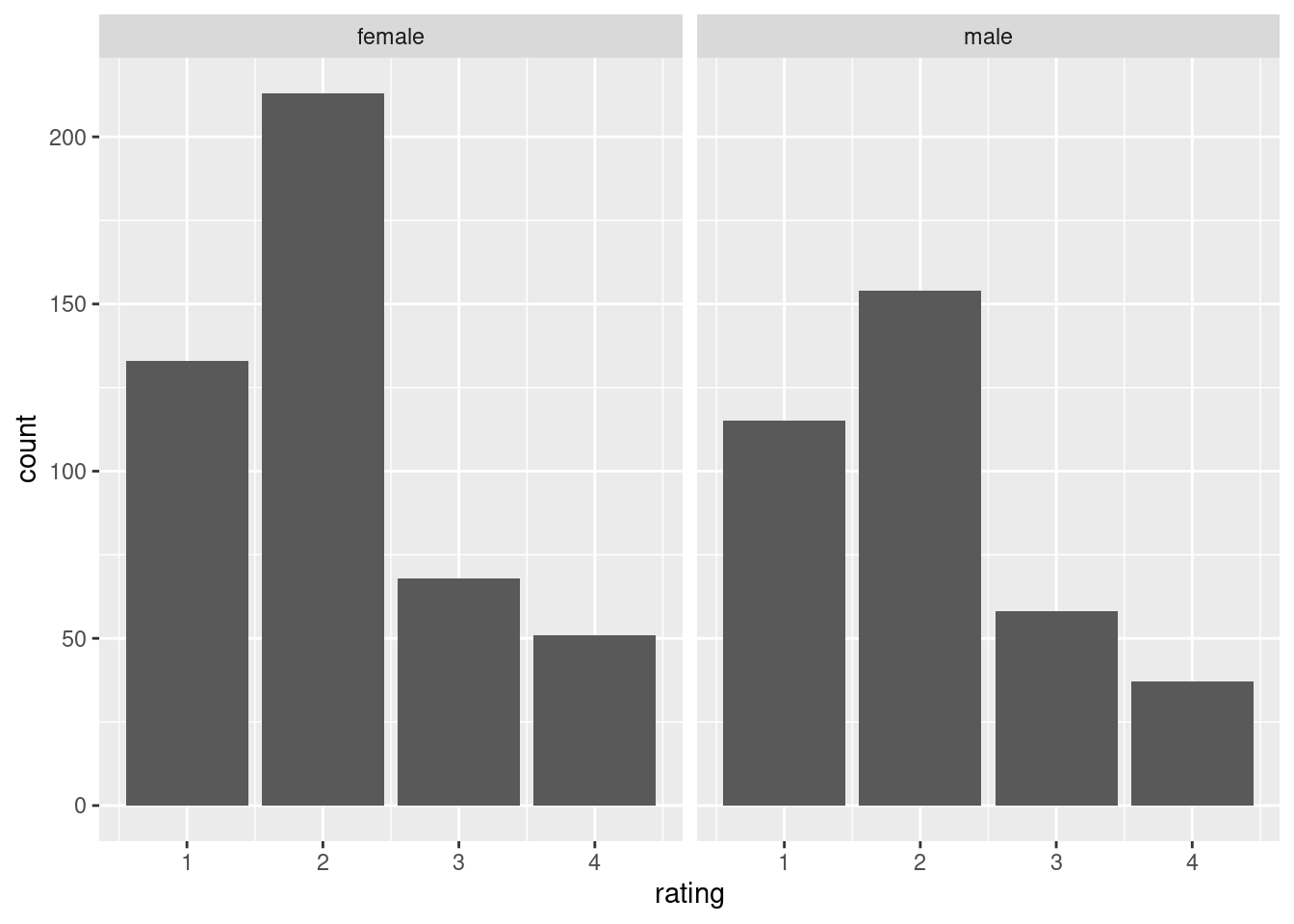
https://www.thearda.com/archive/files/Codebooks/GSS2006_CB.asp
The outcome is attitude towards stem cells research, and the predictor is gender.
Recently, there has been controversy over whether the government should provide any funds at all for scientific research that uses stem cells taken from human embryos. Would you say the government . . .
- 1 = Definitely, should fund such research
- 2 = Probably should fund such research
- 3 = Probably should not fund such research
- 4 = Definitely should not fund such research
Nominal Logistic Regression
Ordinal regression is a special case of nominal regression with the proportional odds assumption.
Model
\[\begin{align} \text{rating}_i & \sim \mathrm{Categorical}(\pi^1_{i}, \pi^2_{i}, \pi^3_{i}, \pi^4_{i}) \\ \pi^1_{i} & = \frac{1}{\exp(\eta^2_{i}) + \exp(\eta^3_{i}) + \exp(\eta^4_{i}) + 1} \\ \pi^2_{i} & = \frac{\exp(\eta^2_{i})}{\exp(\eta^2_{i}) + \exp(\eta^3_{i}) + \exp(\eta^4_{i}) + 1} \\ \pi^3_{i} & = \frac{\exp(\eta^3_{i})}{\exp(\eta^2_{i}) + \exp(\eta^3_{i}) + \exp(\eta^4_{i}) + 1} \\ \pi^4_{i} & = \frac{\exp(\eta^4_{i})}{\exp(\eta^2_{i}) + \exp(\eta^3_{i}) + \exp(\eta^4_{i}) + 1} \\ \eta^2_{i} & = \beta^2_{0} + \beta^2_{1} \text{male}_{i} \\ \eta^3_{i} & = \beta^3_{0} + \beta^3_{1} \text{male}_{i} \\ \eta^4_{i} & = \beta^4_{0} + \beta^4_{1} \text{male}_{i} \\ \end{align}\]
mod <- cmdstan_model("nominal_reg.stan")
mod
## //
## // This Stan program defines a nominal regression model.
## //
## // It is based on
## // https://mc-stan.org/docs/stan-users-guide/multi-logit.html
## //
##
## // The input data is a vector 'y' of length 'N'.
## data {
## int<lower=0> K; // number of response categories
## int<lower=0> N; // number of observations (data rows)
## int<lower=0> D; // number of predictors
## array[N] int<lower=1, upper=K> y; // response vector
## matrix[N, D] x; // predictor matrix
## }
##
## transformed data {
## vector[D] zeros = rep_vector(0, D);
## }
##
## // The parameters accepted by the model.
## parameters {
## vector[K - 1] b0_raw; // intercept for second to last categories
## matrix[D, K - 1] beta_raw;
## }
##
## // The model to be estimated.
## model {
## // Add zeros for reference category
## vector[K] b0 = append_row(0, b0_raw);
## matrix[D, K] beta = append_col(zeros, beta_raw);
## to_vector(beta_raw) ~ normal(0, 5);
## y ~ categorical_logit_glm(x, b0, beta);
## }stan_dat <- with(stemcell,
list(K = n_distinct(rating),
N = length(rating),
D = 1,
y = rating,
x = matrix(as.integer(gender == "male")))
)# Draw samples
fit <- mod$sample(data = stan_dat, seed = 123, chains = 4,
parallel_chains = 2, refresh = 500,
iter_sampling = 2000, iter_warmup = 2000)fit$summary() |>
knitr::kable()| variable | mean | median | sd | mad | q5 | q95 | rhat | ess_bulk | ess_tail |
|---|---|---|---|---|---|---|---|---|---|
| lp__ | -1035.3518437 | -1035.0200000 | 1.7612849 | 1.6160340 | -1038.6900000 | -1033.1300000 | 1.000639 | 3809.196 | 4742.492 |
| b0_raw[1] | 0.4703141 | 0.4697820 | 0.1118201 | 0.1128904 | 0.2877985 | 0.6527007 | 1.001230 | 3667.338 | 5286.149 |
| b0_raw[2] | -0.6762280 | -0.6757360 | 0.1507270 | 0.1497626 | -0.9251864 | -0.4307565 | 1.000439 | 4465.972 | 5274.345 |
| b0_raw[3] | -0.9675208 | -0.9653220 | 0.1672082 | 0.1658889 | -1.2447755 | -0.6988120 | 1.001632 | 4428.634 | 5072.438 |
| beta_raw[1,1] | -0.1760178 | -0.1774040 | 0.1680554 | 0.1646985 | -0.4533714 | 0.1036652 | 1.000391 | 3881.178 | 5200.826 |
| beta_raw[1,2] | -0.0121064 | -0.0135833 | 0.2209685 | 0.2195530 | -0.3762467 | 0.3532682 | 1.000601 | 4376.717 | 5480.247 |
| beta_raw[1,3] | -0.1751981 | -0.1765975 | 0.2540991 | 0.2564196 | -0.5939876 | 0.2370495 | 1.001283 | 4382.617 | 5279.069 |
Compare to brms:
library(brms)
brm(rating ~ gender, data = stemcell, family = categorical(link = "logit"),
    file = "mlogit")
## Family: categorical
## Links: mu2 = logit; mu3 = logit; mu4 = logit
## Formula: rating ~ gender
## Data: stemcell (Number of observations: 829)
## Draws: 4 chains, each with iter = 2000; warmup = 1000; thin = 1;
## total post-warmup draws = 4000
##
## Population-Level Effects:
## Estimate Est.Error l-95% CI u-95% CI Rhat Bulk_ESS Tail_ESS
## mu2_Intercept 0.47 0.11 0.26 0.69 1.00 3990 3108
## mu3_Intercept -0.67 0.15 -0.97 -0.39 1.00 3809 3130
## mu4_Intercept -0.96 0.17 -1.29 -0.63 1.00 4027 3031
## mu2_gendermale -0.18 0.17 -0.51 0.15 1.00 4272 2829
## mu3_gendermale -0.01 0.22 -0.43 0.41 1.00 4141 2902
## mu4_gendermale -0.17 0.25 -0.67 0.34 1.00 3922 2937
##
## Draws were sampled using sampling(NUTS). For each parameter, Bulk_ESS
## and Tail_ESS are effective sample size measures, and Rhat is the potential
## scale reduction factor on split chains (at convergence, Rhat = 1).The estimates are pretty much the same.
Yuan Bo 袁博
Associate Professor of Psychology (Social Psychology)
My research examines the nature and dynamics of social norms, namely how norms may emerge and become stable, why norms may suddenly change, how is it possible that inefficient or unpopular norms survive, and what motivates people to obey norms. I combines laboratory and simulation experiments to test theoretical predictions and build empirically-grounded models of social norms and their dynamics.